Lagrange Multiplier and Dual Formulation

The SVM optimization problem can also be solved with lagrange multipliers. This technique can be used to transform the above constrained optimization problem into a formulation whose solution is equivalent to the above. The reason we would transform the problem in this way is that it allows us to leverage some extremely powerful mathematical techniques. In jargon, we say that the lagrange multiplier solution to the SVM optimization problem re-states the problem in a dual form.

Recall that a constrained optimization problem has the form

$$\begin{array}{ll} \mbox{minimize} & f(x,y)\\ \mbox{subject to} & g(x,y)=c \end{array}$$

where $f$ is called the objective function, and g is called the subjective function. The minimum of the function $f$ subject to the constraint $g - c = 0$, if the minimum exists, is to be found where the gradients of the two functions are scalar multiples of each other. The general Lagrange function can be written as $$\nabla f (x,y) = \lambda \nabla g(x,y)$$

Or equivalently; by setting the gradient of the lagrangian to zero, where the lagrangian is the following function:

$$\mathcal{L}(x,y,\lambda) = f(x,y) - \lambda \cdot (g(x,y)-c)$$

$$\nabla \mathcal{L}(x,y,\lambda) = \nabla f(x,y) - \lambda \nabla (g(x,y)-c) = 0$$

Our particular lagrangian will be written as $$\mathcal{L}(w,b,\alpha)=\frac{1}{2}\mathbf{w}^T\mathbf{w} + \sum_{i=1}^m \left( \alpha_i \left( 1- y_i (\mathbf{w}^T\mathbf{x} + b )\right) \right)$$

Here let the scalar values be written as $\alpha_i$ for $i = 1,\dots, n$. By solving the above problem, we find the following identity: $$\nabla_w \mathcal{L} = \mathbf{w} + \sum_{i=1}^m \alpha_i (-y_i \mathbf{x}_i) =0 \\ \mathbf{w} = \sum_{i=1}^m \alpha_i y_i \mathbf{x}_i \nabla_b \mathcal{L} = \sum_{i=1}^m \alpha_i (-y_i) = 0 \\ \sum_{i=1}^m \alpha_i y_i =0$$

which mean that the correct weights for our problem can be expressed as a linear combination of the data points multiplied by their labels, with some weights . Then we plug $w= \sum_{i=1}^N \alpha_i y_i \vec{x}_i$ back into the Lagrange function, and we find: $$\mathcal{L}(\mathbf{w},b,\alpha) = \frac{1}{2} \left( \sum_{i=1}^m \alpha_i y_i \mathbf{x}_i \right)^T \sum_{j=1}^m \alpha_j y_j \mathbf{x}_j + \sum_{i=1}^m \alpha_i \left( 1- y_i \left( \sum_{j=1}^m \alpha_j y_j \mathbf{x}_j^T \mathbf{x}_i \right) \right)$$

by rearranging the terms, we can simplify it to get. $$\mathcal{L}(\mathbf{w},b,\alpha) = \sum_{i=1}^m \alpha_i - \frac{1}{2} \sum_{i,j=1}^m \alpha_i y_i \alpha_j y_j \mathbf{x}_i ^T \mathbf{x}_j - b \sum_{i=1}^m \alpha_i y_i$$

Since $\sum_{i=1}^N \alpha_i y_i=0$, we can further simplify the above equation by getting rid of the last term: $$\mathcal{L}(\mathbf{w},b,\alpha) = \sum_{i=1}^m \alpha_i - \frac{1}{2} \sum_{i,j=1}^m \alpha_i y_i \alpha_j y_j \mathbf{x}_i ^T \mathbf{x}_j$$

Since we’re minimizing L with respect to w, and w is a function of α, we can restate our minimization problem as the following $$\begin{array}{l l} \underset{\alpha}{\mbox{maximize} }& \sum_{i=1}^m \alpha_i - \frac{1}{2} \ \sum_{i,j=1}^m \alpha_i y_i \alpha_j y_j \mathbf{x}_i ^T \mathbf{x}_j \\ \mbox{subject to} & \alpha_i \geq 0 \ \forall i \\ & \sum_{i=1}^m \alpha_i y_i = 0 \end{array}$$

This is called the dual formulation of SVM, or the dual problem. Any dual problem is always a convex problem. This form can also be solved with quadratic programming, but it changes the problem so that we are minimizing over $N$ variables instead of the original $D$ variables.

A student first learning about SVM needn’t concern himself with the exact details of this problem. It is important to understand what the $N$ variables, $\alpha_i$, correspond to . They decide how ‘important’ each point in our training set is. There is one alpha for every data point in the training set. The solution of the minimization problem assigns a high alpha to points that are very important, and a low alpha to points of low importance. Conceptually, the points with high alpha values, or high importance, are the data points that are closest to the decision boundary. In practice, almost all alpha values in the solution will go to zero. The training points with non-zero alphas are called the support vectors of the classifier.

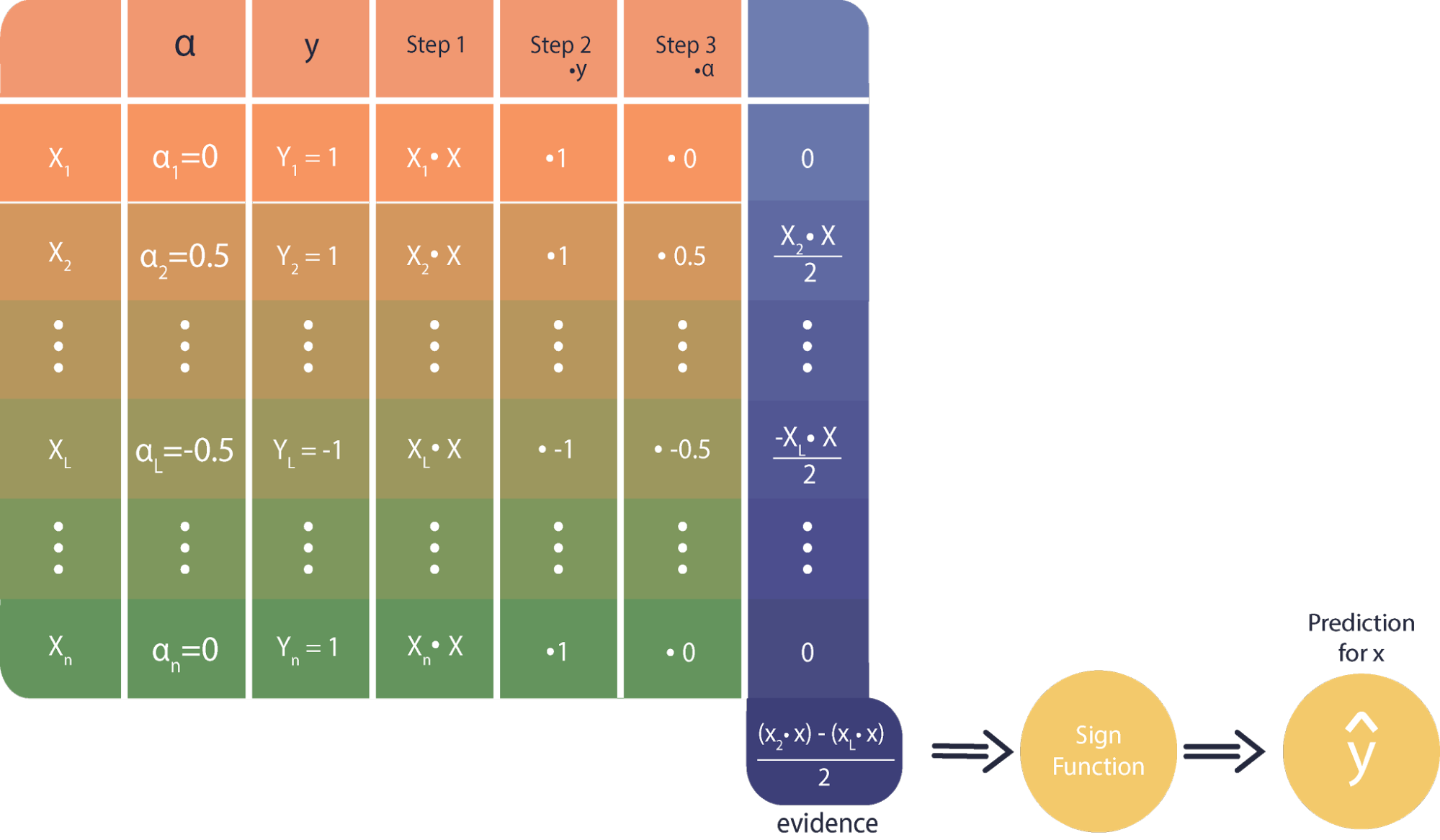
After training in dual form, our classification rule becomes $f(\mathbf{x}_i) = \mbox{sgn} \left( \sum_{i=1} \alpha_i y_i \mathbf{x}_i^T \mathbf{x}_j \right)$

where xi is the ith training point in our dataset, x is the new point being classified, and yi is the true label of xi. The dual form SVM approach changes the logic of both the training problem and the classifier rule. Instead of finding an explicit decision boundary, we have found a set of values over our training points that we can use to describe how ‘representative’ each training point is of its class.

The logic of the classifier function has changed in a corresponding way. Instead of finding whether some new point is above or below the decision boundary, we take the dot product between between the new point and every training point, combine these values with the importance and class sign of the training points, and then sum over these values. Because only a small set of training points will receive a non-zero alpha, we actually only need to store a subset of our training data.

The classifier is easy to understand if we recall that the dot product is a similarity function between two vectors. The classifier combines the similarities between the test point and all our support vectors with the classes and importance values of our support vectors.

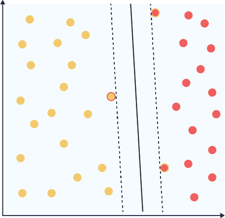
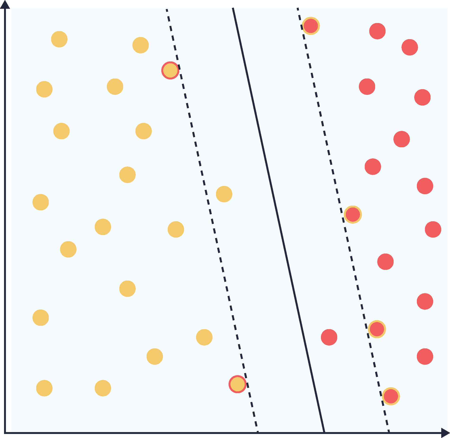
Our classifier here has many conceptual similarities to the KNN classifier, (LINK KNN wiki) however, it does not suffer from the usual problems of KNN. We don’t need to store an entire training set to classify, because only a subset of our training points have non-zero importance. The image below shows two SVM classifiers in dual form, each trained with a different value of the slack parameter C. The support vectors of either class are highlighted in both images. In the first case, C was chosen to be 5, there are 3 support vectors, and the margin is relatively small. In the second image there are 6 support vectors, C was chosen to be 2, and the margin is significantly larger. The second case has two ‘in margin’ points.