Hard Margin for linearly separable data

The hard margin is the oldest and simplest formulation of SVM. It assumes that the dataset is linearly separable by class. We will drop this assumption in later sections, but it is useful to consider this case when first learning SVM. Suppose we are given a training dataset of m points of the form,

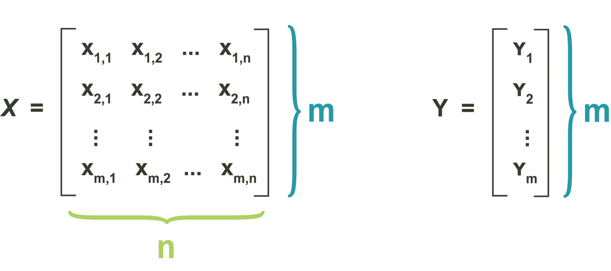
where each training label $y_i$ is either 1 or -1, indicating the class to which the point xi belongs. Each data point $x_i$ is a m-dimensional real vector. Assume that there exists some set of linear decision boundaries for which all points are correctly separated. We want to find the maximum-margin decision boundary that divides the group of data points for which $y_i = 1$ from the group of points for which $y_i = -1$, such that the distance between the hyperplane and the nearest points from either group is maximized.

Any hyperplane can be written as a set of all points x that satisfy $\mathbf{w}^T\mathbf{x} + b = 0$

where $w$ is a vector normal to the hyperplane. It is important to remember that the ratio of parameters $\frac{b}{ \left| \left| \mathbf{w} \right| \right| }$ determines the intercept of the hyperplane from the origin along the normal vector $w$. If the training data are linearly separable, we can define two parallel hyperplanes that straddle the nearest point of either class. We will define our two parallel hyperplanes as those that run through the nearest point of either class, such that for some $w$ and $b$, $\mathbf{w}^T\mathbf{x} + b = 1$ and $\mathbf{w}^T\mathbf{x} + b = -1$

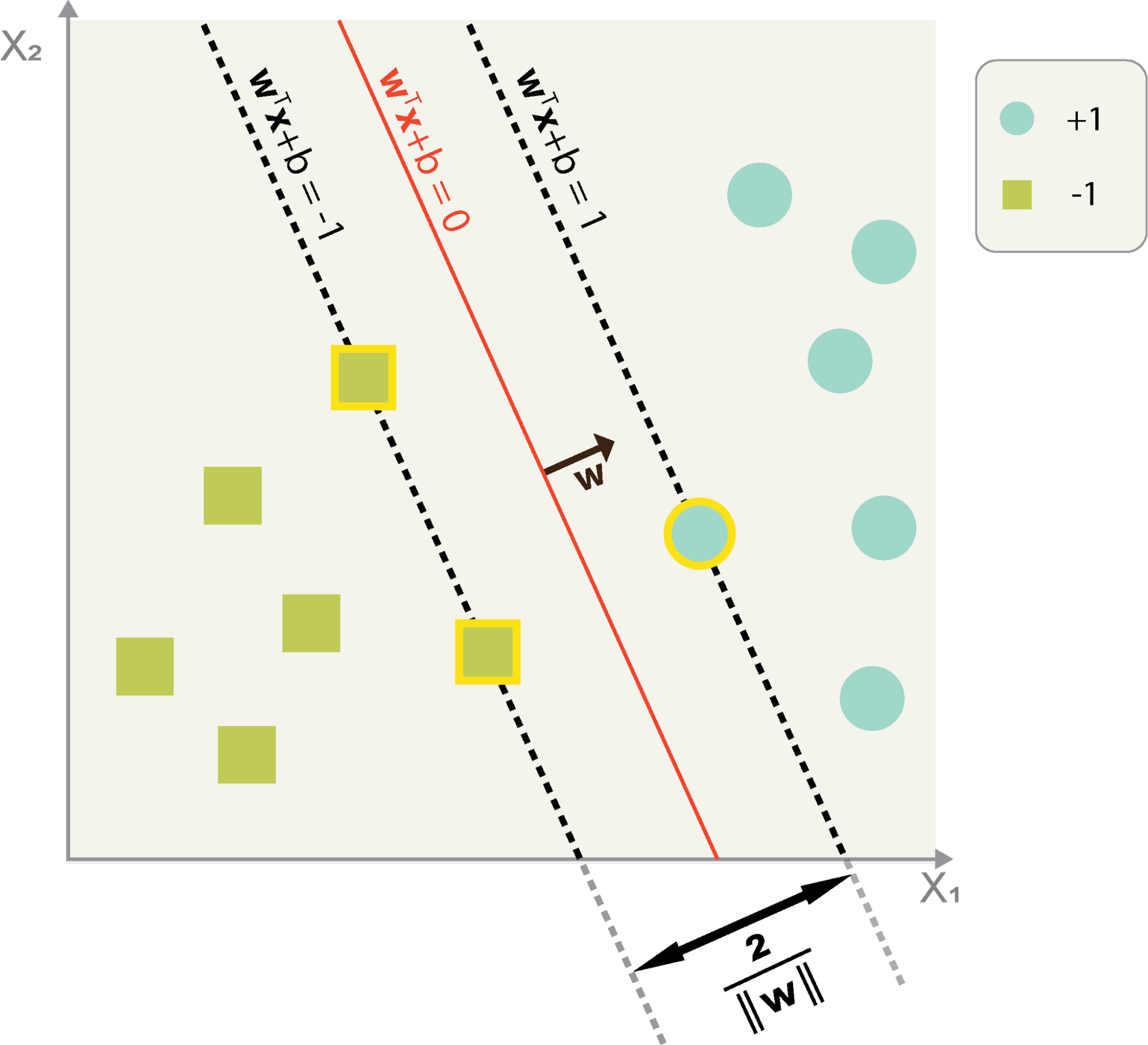
We define our decision boundary as the halfway mark between these two boundaries, specifically, as the set of points in the feature space that satisfy $\mathbf{w}^T\mathbf{x} + b = 0$ By defining our decision boundary as the halfway mark of these two hyperplanes, we are guaranteeing that the boundary is equidistant from the two classes.

The maximum-margin decision boundary will run through the halfway mark between our two ‘boundary’ hyperplanes. Our goal then, is to define and maximize the distance between these two boundaries as a function of the weights and biases. The distance between these two ‘edge’ hyperplanes along their common normal vector can be defined as follows.

$$\frac{b + 1}{ \left| \left| \mathbf{w} \right| \right|} - \frac{b -1 }{ \left| \left| \mathbf{w} \right| \right| } = \frac{2}{ \left| \left| \mathbf{w} \right| \right| }$$

Thus, to maximize the distance between the planes is to maximize $2‖w‖$, which is equivalent to minimizing $‖w‖$. The above derivation shows that of the infinite possible decision boundaries with perfect training accuracy, the one with the largest margin is the one with the smallest magnitude of weights. Because our derivation is based on a pair of margin-edge hyperplanes, our resulting optimization problem has to make use of the same definitions. This will be shown concretely next.

The SVM prediction function, is written as $$\mathrm{sgn}(x) = \begin{cases} -1 & \mbox{if} \ x >0 \\ 0 & \mbox{if} \ x = 0\\ 1 & \mbox{if} \ x < 0 \end{cases}$$ $$f (\mathbf{x}) = \mathrm{sgn}(\mathbf{w}^T\mathbf{x} + b )$$

which allows us to formally write a condition for perfect classification accuracy: $$\forall i, y_i (\mathbf{w}^T\mathbf{x} + b ) \geq 0$$

which can be read as ‘for all points in our dataset, the label and the classifier input are the same sign.’ $$\forall i, y_i (\mathbf{w}^T\mathbf{x} + b ) \geq 1$$

Because our minimization criteria was derived by defining two margin-bonding planes, our problem’s conditions need to reflect this. So, we use the following constraint for perfect accuracy in our framework instead the standard one above: $$\forall i, y_i (\vec{\mathbf{w}} \cdot \vec{\mathbf{x}} + b ) \geq 1$$

where each point is not only accurately predicted, but is also outside of the margin as we’ve defined it. If we don’t define the points as being outside the margin, then the minimization criteria we’ve defined won’t apply to them.

Putting together all of the above, we turn the abstract concept of the SVM problem into a concrete, constrained optimization problem: $$\underset{\mathbf{w}} {\mbox{arg\ min} } \frac{1}{2} \left| \left| \mathbf{w} \right| \right| \mbox{subject\ to} \ y_i (\mathbf{w}^T\mathbf{x} + b ) \geq 1\ \forall i$$

$$\begin{array}{ll} \underset{\mathbf{w}} {\mbox{minimize}} & \frac{1}{2} \left| \left| \mathbf{w} \right| \right| \\ \mbox{subject\ to} & \ y_i (\mathbf{w}^T\mathbf{x} + b ) \geq 1\ \forall i \end{array}$$ where the bias term $b$ is given, after solving for $w$, by $$b = -\frac{max_{i:y_i=-1} w \cdot x_i + min_{i:y_i = 1 w \cdot x_i}}{2}$$

This problem is a convex problem, and can be solved using any quadratic programming function. Once the set of weights and bias have been found, the classifier as shown above can be used to predict on any new point.

Any formulation of the SVM that uses the native weight parameter $w$, as in the above, and minimizes over this parameter, is said to be in primal form. Another form of the problem arises when we use lagrange multipliers to minimize the function in a closed form solution. This process yields the famous dual form formulation, discussed below. The following section discusses extending the SVM to non-linearly separable data, which also allows for more control over the regularization process. This is done by laxing the constraint that all points need to be correctly classified and ‘past the margin.’

For non-linearly separable boundaries, the classic perceptron simply will not work, and other AN methods still have the same issue as above. However, the SVM can be equipped with a soft-margin extension, which produces considerably improved performance over other AN methods. Soft-margin SVM is treated in detail in a later section.