How it Works?
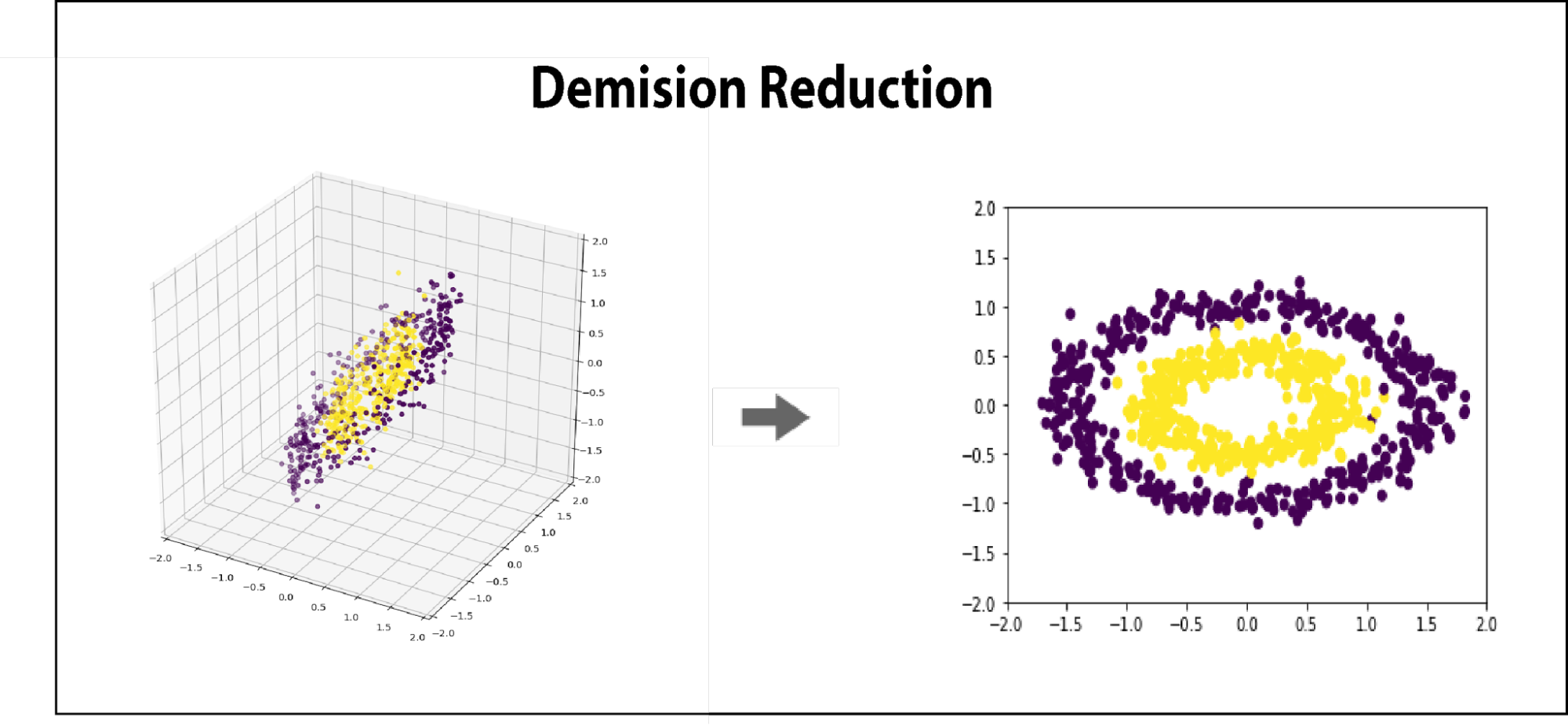
PCA finds the direction of greatest information by computing the directions of greatest variance, and then projecting the dataset onto vectors that correspond to those directions.
Consider a standard unlabelled dataset, given by the matrix X.
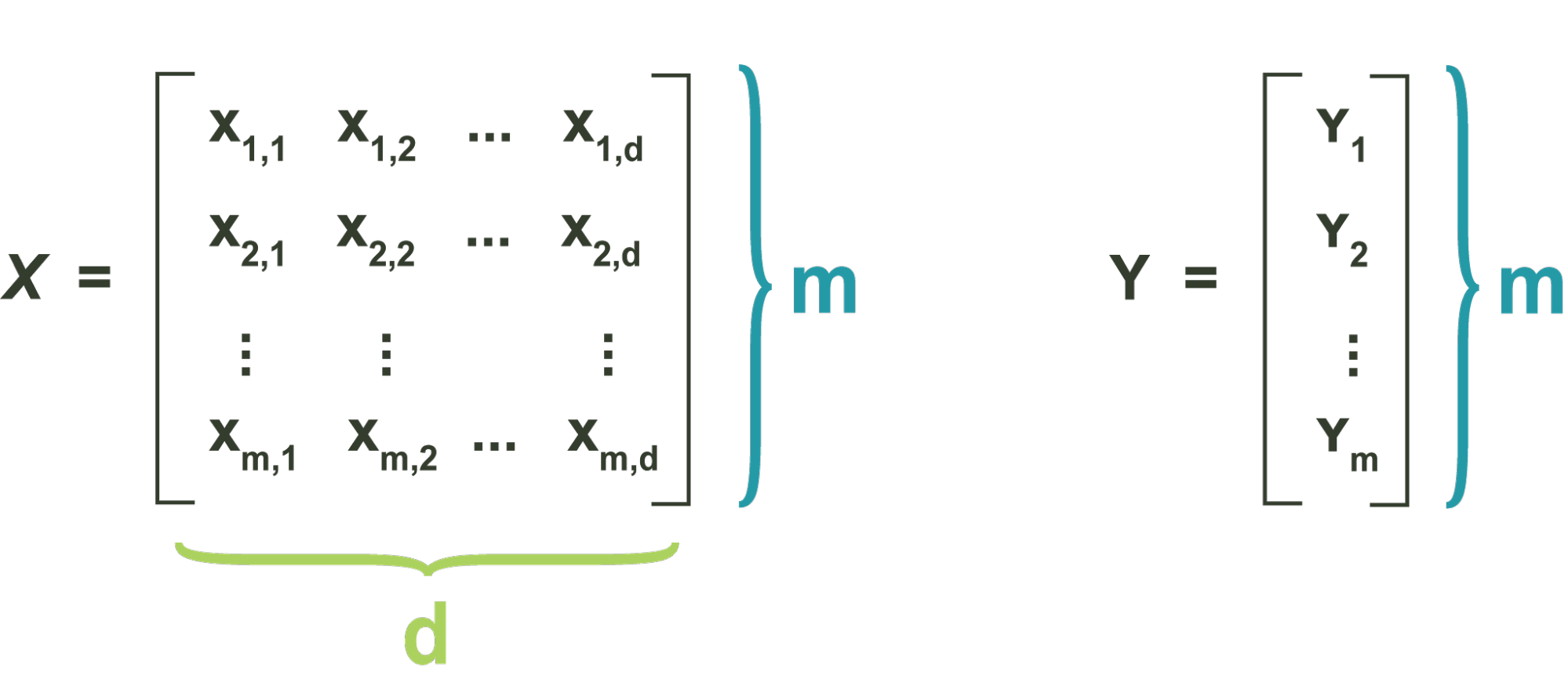
X is composed of m data vectors, which are the rows of the matrix, each in a d-dimensional feature space.
The directions of greatest variance in a dataset are given by the eigenvectors of the covariance matrix of that dataset, which in turn is defined by variance and covariance of all the dimensions in the dataset. Variance is a measure of the spread of one variable. Covariance is a measure of the spread between two variables. Formally, the two are similar:
Here, and refer to the mean of and , respectively.
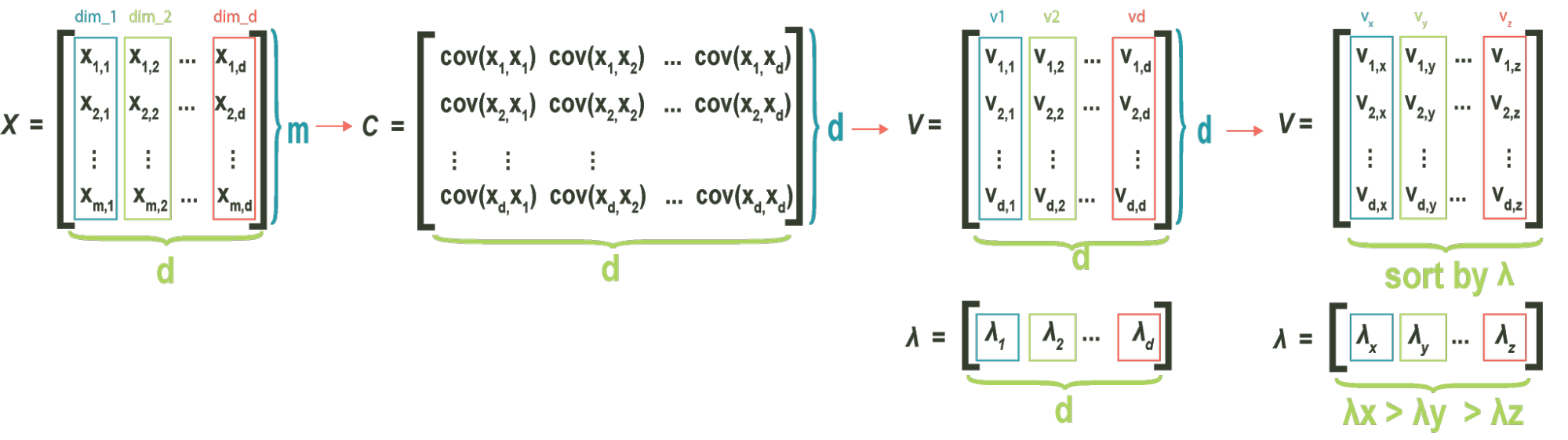
The **covariance matrix**, which is central to PCA, is composed of all variance and covariance measures of our dataset. The element of the matrix is the covariance between i-th and j-th variable. For 3 dimensions, the covariance matrix C is given by:
Where refers to . Notice that for a D-dimensional dataset, we will always have a DxD covariance matrix, given by
A matrix A has an **eigenvector** v with the associated **eigenvalue** lambda if
Where A is a square matrix, v is a column vector, and lambda is a scalar. For an NxN square matrix, there are always N eigenvectors with associated eigenvalues for that matrix.
The **eigenvectors** of the **covariance matrix** correspond to the directions of ranked variance described above. Specifically, the **eigenvector** of the **covariance matrix** with the largest eigenvalue always points to the direction of greatest variance in the data.. The **eigenvector** with the second largest eigenvalue points in the direction of second largest variance, orthogonal to the first eigenvector. This pattern continues, where the third eigenvector points in the direction of third largest variance, orthogonal to both the first and second eigenvectors, and so on.
Once the **eigenvectors** are found, it is customary to sort them by associated **eigenvalue**. Sorting the vectors makes future computation extremely easy, as the index of each vector corresponds to its ranked importance.
Projecting a dataset onto a new axis can be accomplished with matrix multiplication. Specifically, for a matrix D, with rows as dimensions and columns as data points, along with a basis V, whose columns are directions we are mapping onto, the re-orientation, or projection, T, of the dataset D by the columns of V is given by the product:
Where X is the data matrix, V is the matrix of ranked eigenvectors as columns, and C is the dataset re-defined in a space where each dimension is ranked by variance.
Because the eigenvectors are ranked by variance, they inform the user as to which directions can be dropped once the data has been redefined in component space. This means that the resulting matrix, C, which has the same shape as X, can be reduced by N dimensions of least variance, simply by removing it rightmost N columns.
Because the dimensions of C are ranked by variance, as long as we are removing vectors from the right, we can be confident that we are minimizing the change in overall data structure per dimension removed.
The data can be left in the projected space, called the component space, or can be projected back into its original dimensionality, a process called reconstructing. If a reduced dataset is reconstructed back into its original basis, it will be, in its original space, flattened along the directions of least variance. Reconstructing a data set is often referred to as de-noising.