Step By Step Explanation

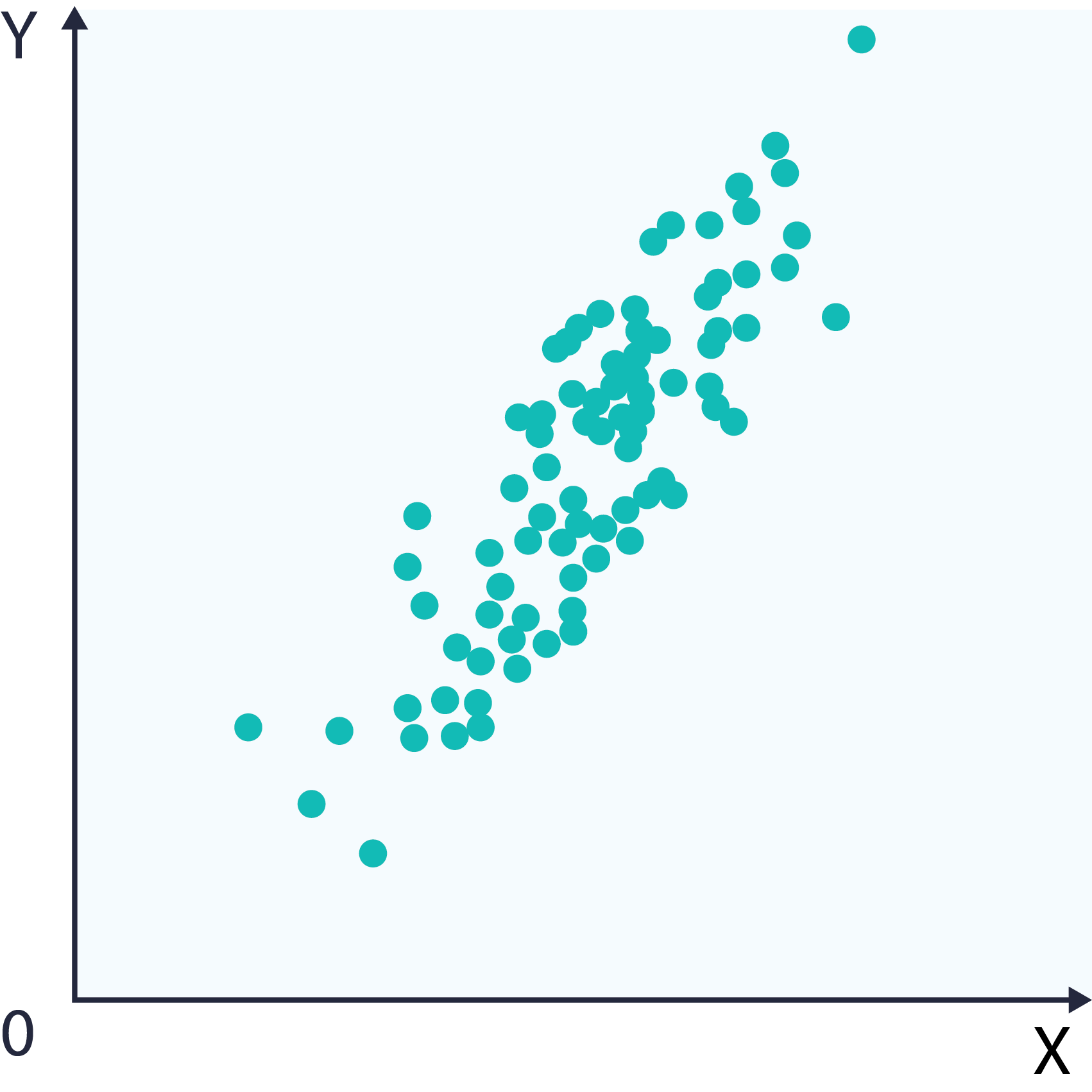
We can distill PCA into the following steps: Let our original data be the following plot

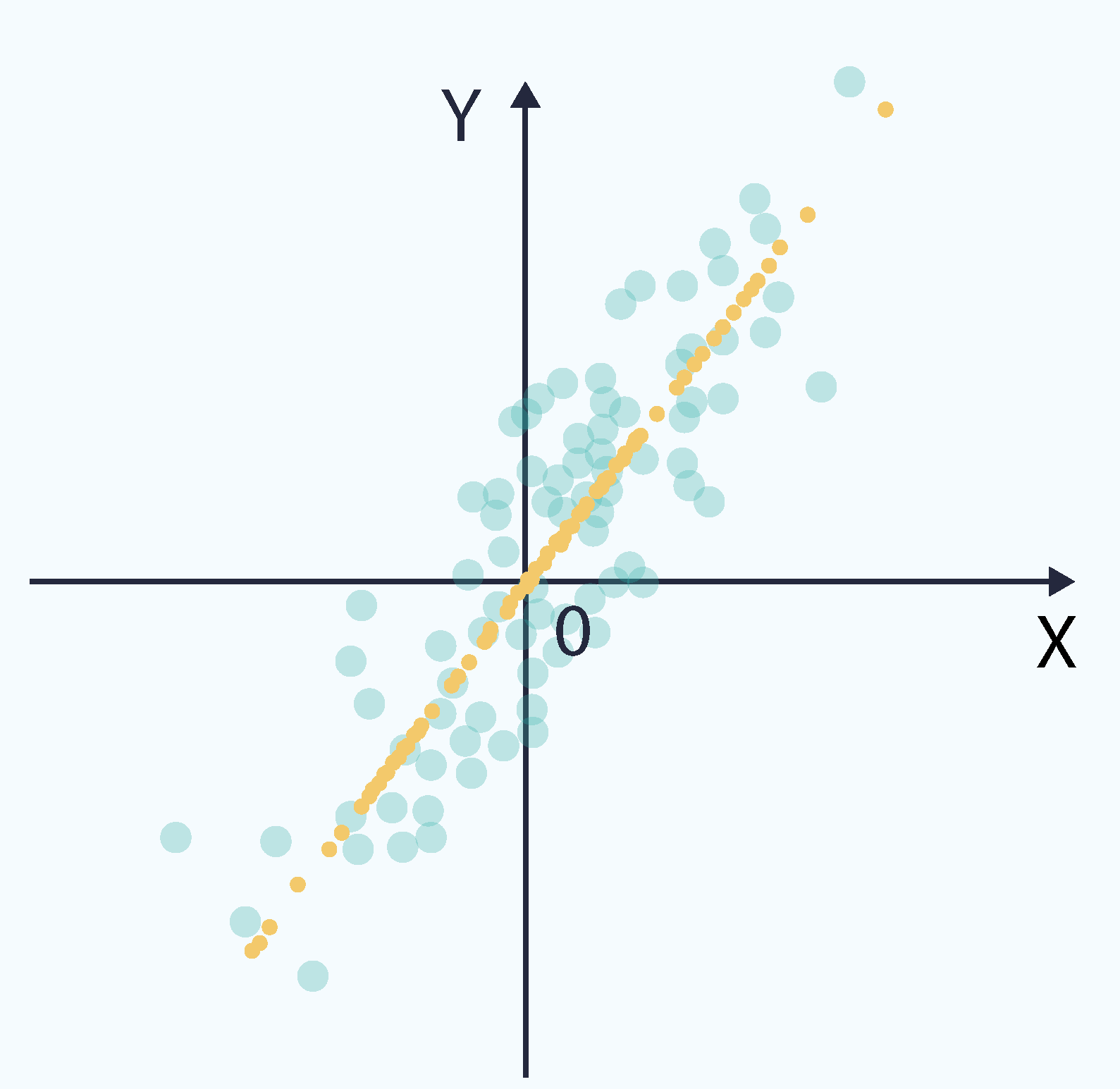
1 – Subtract the mean vector from each of the dimensions

This produces a dataset whose mean is zero called Zero Mean Data. Subtracting the mean simplifies the process of calculating the covariance matrix. This yields the plot on the right (note the axis label):

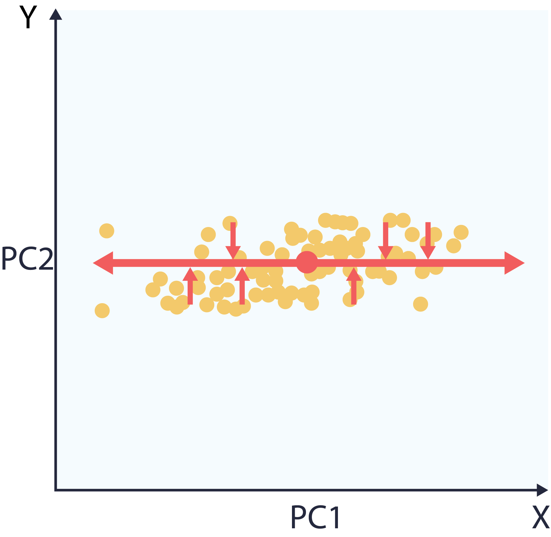
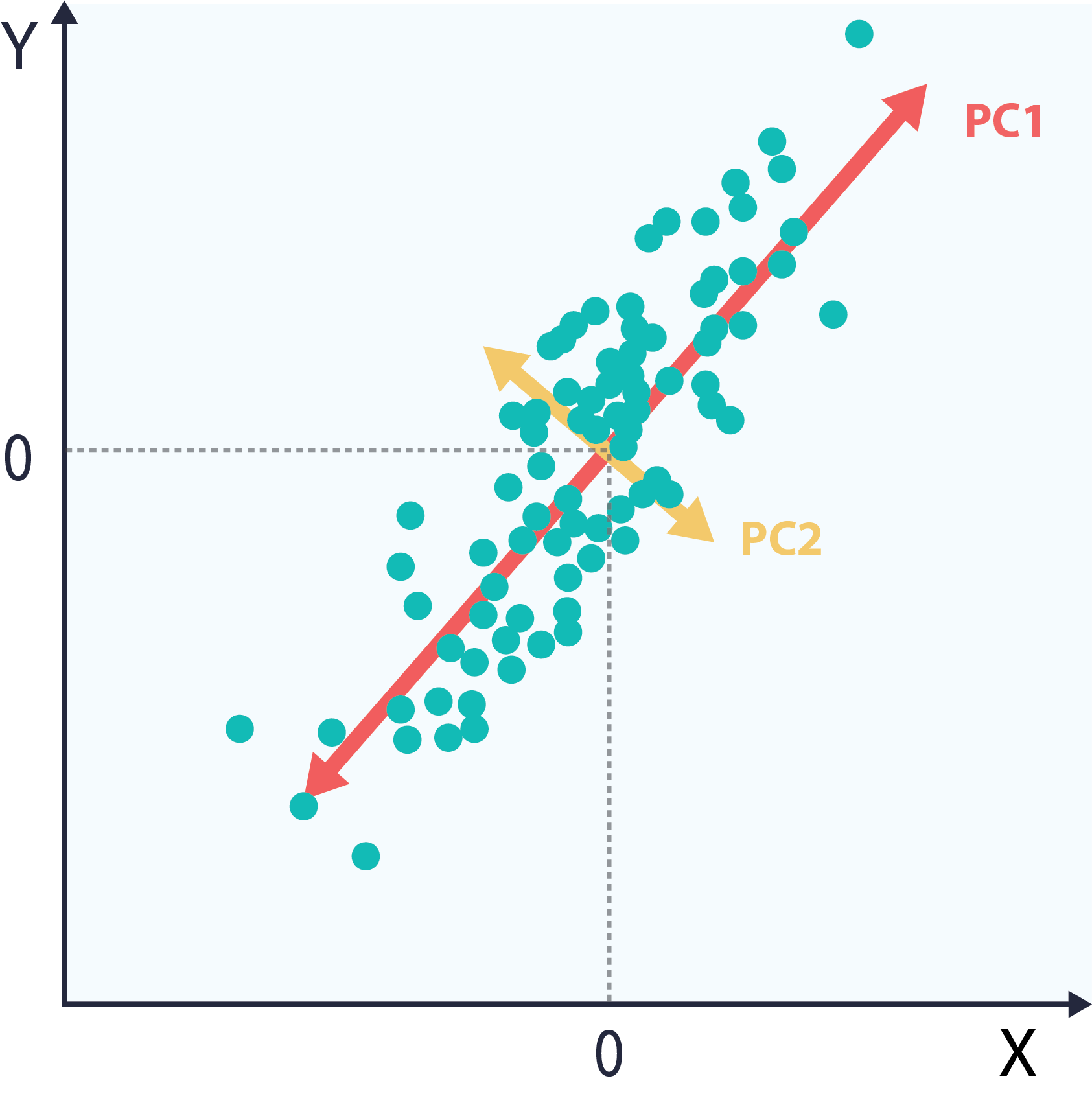
2 – Compute principal components by calculating and ranking by eigenvalue the eigenvectors of the covariance matrix

As described above, the eigenvectors and eigenvalues of the covariance matrix correspond to orthogonal directions of variance. When ordered by eigenvalue, they form the principal components. The following plot shows the same dataset, with the principal components directions highlighted in red and green

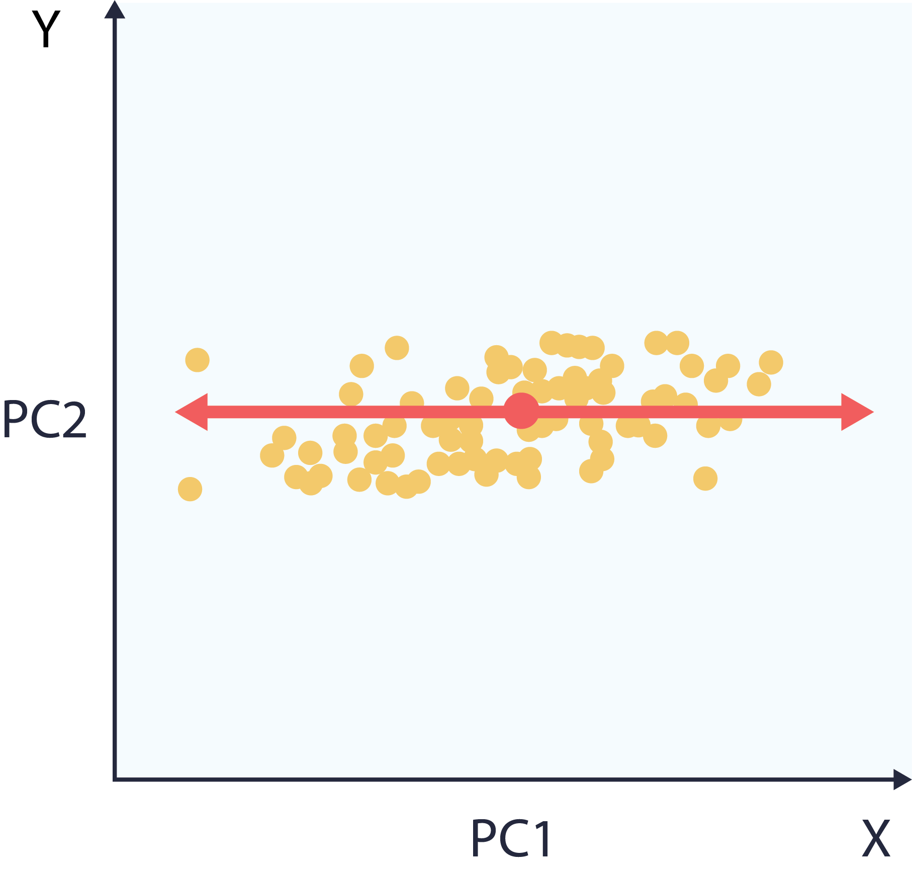
5 – Project the data into component space.

This makes it so that the dimensions of our dataset are now ranked by variance. Specifically, the x-axis now aligns with widest spread, the y-axis with narrowest.

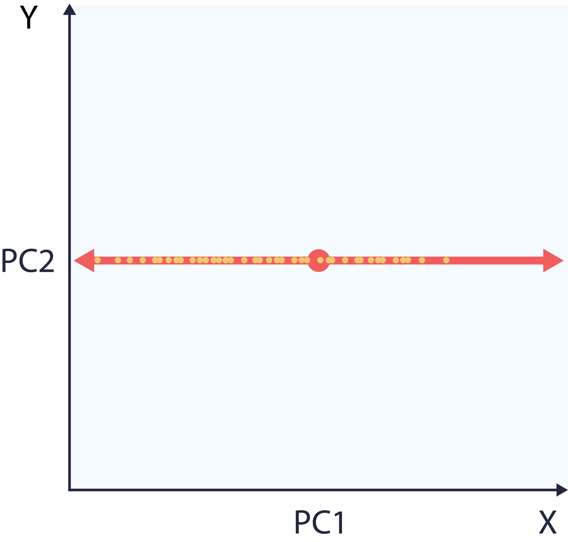
6 – Choose and apply application.

At this point, the user can choose to reduce dimensions or denoise. Reducing dimensions is just a matter of dropping values of the least informative directions in in component space. This means a smaller dataset that preserves the data’s original structure, seen in the following plot. Note that the dataset on the right is one dimensional, representable with a single vector.