Common kernels

Summary of Inner-Product Kernels

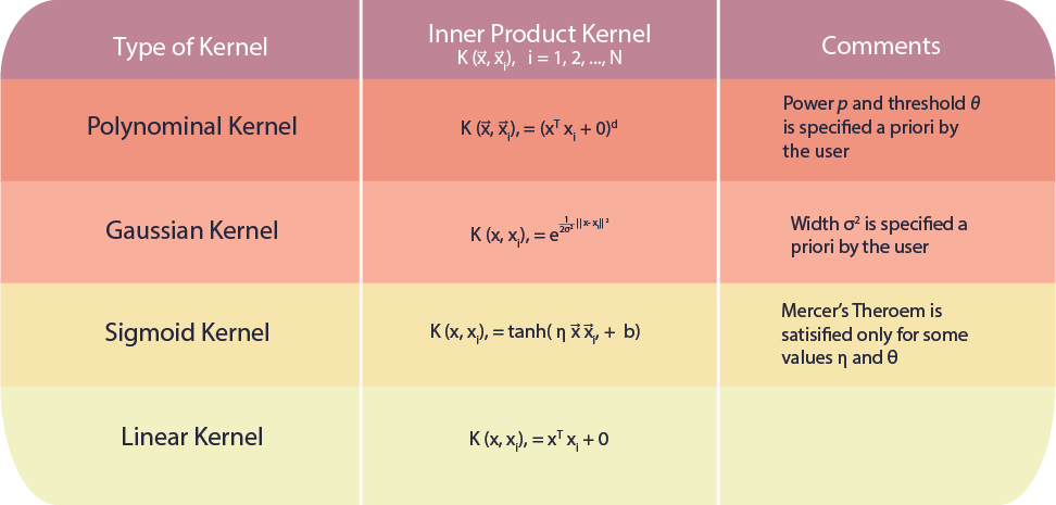
The above table shows some common kernels. Although some kernels are domain specific there is in general no best choice. Since each kernel has some degree of variability in practise there is nothing else for it but to experiment with different kernels and adjust their parameters via model search to minimize the error on a test set. Generally, a low polynomial kernel or a Gaussian kernel have shown to be a good initial try and to outperform conventional classifiers.

Polynomial Kernel

In this section we show that using polynomials as a basis can also be computed using a kernel. This is an example of how the kernel can be easier to compute, instead of computing the expansion into all possible polynomial terms. $$\begin{align*} w_{1}x+w_{2}x^{2}+w_{3}x^{3}\end{align*}$$ We could model the introduction of polynomial terms as a function from vectors x to vectors in a higher dimensional space $$\begin{align*} \Phi(x) =[x_{1},x_{1}^{2},\ldots x_{1}^{p},\ldots x_{n},x_{n}^{2},\ldots,x_{n}^{p}]\end{align*}$$ where p is the order of our polynomial. If we replace each row of X (examples in the data) with $\Phi(x)$, note that in the dual, we would have a matrix of inner products $\Phi(x)^{T}\Phi(y)$. It turns out that for certain values of the expansion, we can compute the dot products directly, instead using a kernel function. $$\begin{align*} K_{poly}(\mathbf{x},\mathbf{y}) & =(\mathbf{x}^{T}\mathbf{y}+1)^{p}\end{align*}$$ For $p=2$, the polynomial kernel is: $$\begin{align*} (x^{T}y+1)^{T}(x^{T}y+1)\end{align*} \begin{align*} y^{T}x^{T}xy+2x^{T}y+1\end{align*}$$ note that we can rearrange terms since $x^{T}x$ is a scalar: $$\begin{align*} \mathbf{x^{\mathit{T}}}\mathbf{x}\mathbf{y^{\mathit{T}}y}+2\mathbf{x^{\mathit{T}}y}+1\end{align*}$$ Which is the same thing as $$\begin{align*} [x_{1},x_{1}^{2},\ldots x_{1}^{p},\ldots x_{n},x_{n}^{2},\ldots,x_{n}^{p}]^{T}[y_{1},y_{1}^{2},\ldots y_{1}^{p},\ldots y_{n},y_{n}^{2},\ldots,y_{n}^{p}]\end{align*}$$

Gaussian Kernel

This is the most widely used kernel. This kernel measures similarity as $$\begin{align} k(i,j)=\exp^{ \frac{\left|\left|\mathbf{x}_i-\mathbf{x}_j \right|\right|_2^2} {\sigma} } \end{align}$$

and there are a few ways to think of this kernel. One is as a radial basis function neural network, with fixed weights: it centers one basis function at every training data point.

Often in the literature it's referred to as a projection into infinite-dimensional space. The basic argument is that the kernel matrix extracted will always be full rank, so that you can always incorporate additional points. Recall that a full-rank kernel is positive definite.

Another explanation is that the points are lifted to a hypersphere, or actually nonnegative orthant of a unit hypersphere. The maximum of the Gaussian kernel occurs when we measure the distance between a point and itself, where the expression evaluates to $1$. This means the length of each data point is $1$, placing it on the sphere. Distances are going to be bounded between $0$ and $1$, because they cannot be negative. This also ensures that the kernel has to be positive definite.

The gaussian kernel contains all functions, because it is full rank. It contains all linear decision boundaries It contains all polynomials, for example if you were doing regression, using the gaussian kernel would give you a polynomial shaped prediction. It contains the constant function, which means that the bias term is unnecessary.

Random Kitchen Sinks

Kernel methods don’t scale well beyond a few thousand points, because the main computational work is inverting the kernel matrix, which grows with the number of points. However, we might want to train a nonlinear method like a support vector machine on millions of points. We have seen in the support vector machine that a linear support vector machine can be trained very quickly using an algorithm like PEGASOS.

This suggests the following idea: use a large number of fixed, but random features. Random features multiply the input datapoint by a random weight vector, then threshold based on the sign. This is the same thing as using a randomly wired neural network, without learning, and this method is very old, for example appearing in the very first paper on perceptrons in 1958. The surprising things are that 1) it works very well in practice (and theory) and 2) with careful attention to the choice of random distribution, you can approximate kernels such as the Gaussian Kernel.

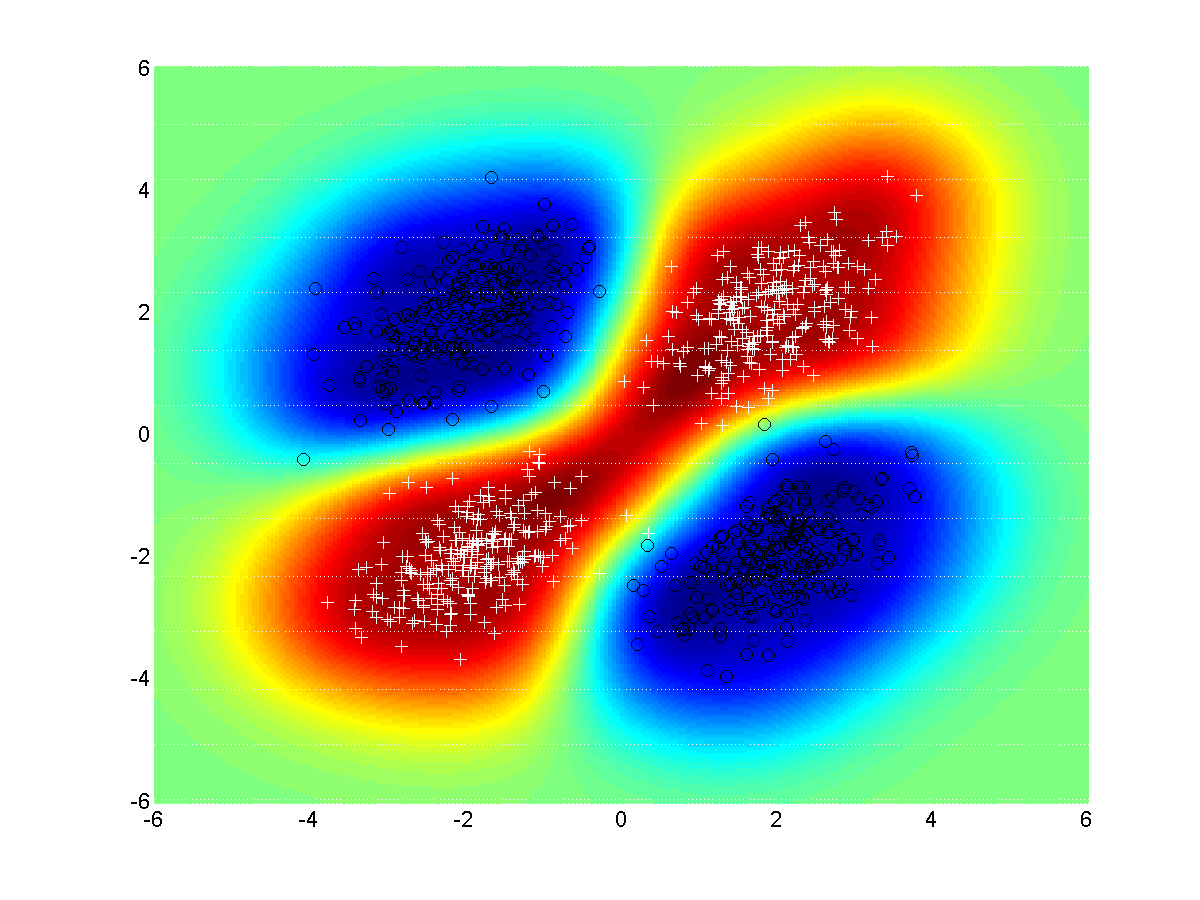
An example is shown below. The data points form two different classes, $+$ and $0$, and we can see in the figure that a nonlinear decision boundary is necessary. The colors plot the decision surface: recall that the prediction rule is thresholding the dotproduct $x^t w$ to give class $1$ or $-1$. Points which are more red are in one class, points in blue are in the other class. The figure below used the gaussian kernel:

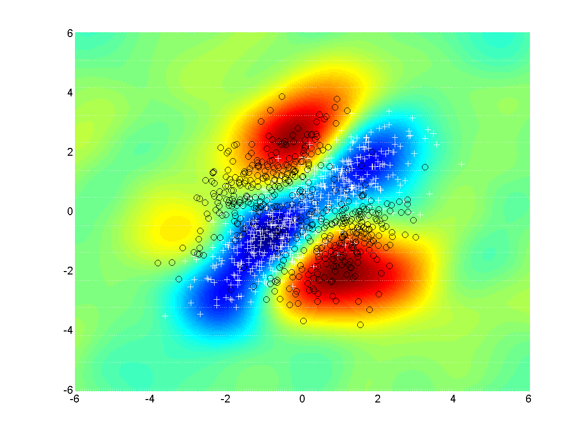
In the next figure, we plot the same decision boundary, but now using a randomly wired input layer (random kitchen sink features). Although not as smooth, this network can still solve the XOR problem.