Probability Notation
Probability theory make extensive use of set notation, so let us first introduce some relevant set operation notation and terminology. Suppose we have a randomized experiment that has some fixed set of possible outcomes. The set of all possible outcomes is called outcome space, denoted as . Think of this as a collection of all possible occurrences within our framework.
For example, The outcome space () for rolling one 6-sided dice is with all equal probability and for rolling two 6-sided dices is . The outcome space () for tossing a coin is {Head, Tail}.
Probability is based on axioms for events, is a formal way of assigning numbers based on the relative number of events of a certain type within the outcome space.
1. {% math %}0 \leq P(A) \leq 1{% endmath %} for all event {% math %}A \in \Omega{% endmath %}
2. {% math %}P(\Omega)=1{% endmath %}
3. {% math %}P(\varnothing)=0{% endmath %}
Events within our space of possible outcomes are not the same ‘size.’ The events with ‘larger’ areas in the set of outcomes have a larger probability. The probability of an event is just the percentage of the outcome space it takes up. A circumstance where the set of outcomes being modelled all have the same probability is called uniform.
Probability is ultimately a measure of relative ‘sizes’ of possible events. , in the above, refers to all possible occurrences within whatever framework we’re modeling. In the case of a die, it is the set of all possible roll outcomes, in which case it would have six elements. In the case of a game of roulette, it is the set of all possible landing outcomes, and would have thirty-eight elements. In the case of two die rolls, we can write the outcome space as all possible pairs of roll outcomes, which would consist of thirty-six possible outcomes. These axioms have extremely simple interpretations. Axiom one just defines the nature of probability, that any event is either impossible, somewhat possible, or necessary, and states that a probability value must be between , for impossible, and , for certain.
The notation can be read as “The probability that an event is within the space of all possible events.” Read in this way, the probability is intuitively certain. can be read as “The probability that an event is outside the space of all possible events occurs.” Intuitively, this should have a probability of . If we encounter an outcome that is not within our , then our model is too weak to describe the outcome.
- Basic Set Notation Reference Table
| Notation | Meaning |
|---|---|
| empty set - impossible event | |
| outcome space - certain event | |
| A union B, A or B | |
| or | A intersect B, A and B |
| or | A’s complement, Not A |
Event Probability Visualization
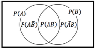
The Venn Diagram is a very useful visualization of the relationships between events. We will be using this venn diagram to illustrate the concepts. For all examples below, the left circle is the event A, and the right circle corresponds to event B. Our is the entirety of the rectangle.
We can visualize the probability of an event as the ratio between the area corresponding to that event and the area of the whole output space. P(A), for example, is the area of the left circle, divided by the area of the whole rectangle. P(B) = P(A) because the two circles are equal size.
We can ask questions like ‘what is the probability that event A didn’t occur’ using this sort of graph as an aid. The probability that event A didn’t occur is the relative area of the whole rectangle minus the area of A, divided by the area of the whole rectangle. This is called the complement of A, and it as well as many other simple probabilities are visualized in the proceeding section.