Markov Chain

A Markov chain is a probabilistic graphical model (PGM) with a chained, directed structure, where any node depends directly only on the preceding nodes in the chain, meaning that this PGM fulfills the markov property. A Markov chain consists of two basic elements. When we say that we have a markov chain, we mean that we have the following two things defined, a state space, which is the set of all possible states of the system (e.g. sunny or rainy weather) and a probability transition function that describe the probability of moving to any of the possible states, given the current state.

The states can be considered as the events in our model. They correspond to the nodes of our PGM. The probability transition function is the probability of transitioning from a given event to the next one of interest. It corresponds to the branches of PGM. If the state space is finite we can define the probability transition matrix $P$. Consider a Markov chain with the state space consisting of three states: $X_1, X_2 and X_3$.

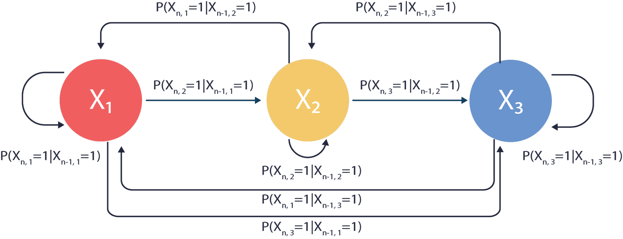
Probability of transitioning from one state to another are shown next to the respective branch. These probabilities are written in a binary notation. To understand this notation the useful way is to think of a vector Xn assigned to the nth state of the Markov chain. For the Markov chain above this vector is $$\vec{X}_n=\begin{bmatrix} X_{n,1}\\X_{n,2}\\X_{n,3} \end{bmatrix}$$

Only one entry of this matrix can ever be one, while others can only be zero. The non-zero entry of the vector corresponds to the state of the Markov Chain at the nth step. Therefore if at the 3rd step the Markov Chain is at the 2nd state the vector $X_3$ is

$$\vec{X}_3=\begin{bmatrix} 0\\1\\0 \end{bmatrix}$$

The probability of the sequence of events $X_1,X_2,X_3,X_1$ given that we start at $X1$ is $P(X_{n,1}=1,X_{n-1,3}=1,X_{n-2,2}=1,X_{n-3,1}=1)=P(X_{n-1,1}=1)*P(X_{n,2}=1|X_{n-1,1}=1)*P(X_{n,3}=1|X_{n-1,2}=1)*P(X_{n,1}=1|X_{n-1,3}=1).$

The numbers that are assigned to each branch exiting the state add up to one, because transitions are mutually exclusive events and they form the sample space for the event of transitioning from the current state. The Markov Chain above has a finite state space so we can construct a transition matrix P that corresponds to the Markov Chain shown above.

$$\begin{bmatrix} P(X_{n,1}=1|X_{n-1,1}=1) & P(X_{n,2}=1|X_{n-1,1}=1) & P(X_{n,3}=1|X_{n-1,1}=1)\\ P(X_{n,1}=1|X_{n-1,2}=1) & P(X_{n,2}=1|X_{n-1,2}=1) & P(X_{n,3}=1|X_{n-1,2}=1)\\ P(X_{n,1}=1|X_{n-1,3}=1) & P(X_{n,2}=1|X_{n-1,3}=1) & P(X_{n,3}=1|X_{n-1,3}=1) \end{bmatrix}$$ Each state has a stationary distribution associated with it. If we have a vector of all stationary distributions $π$ then by definition this vector satisfies the relationship $\textbf{P}\vec{\pi}=\vec{\pi}$ This means that the stationary distribution vector is an eigenvector of the transition matrix with an eigenvalue of 1. The stationary distribution of the state is a reciprocal of the expected value of steps required to return to the same state given that you start at that state. The greater the stationary distribution is, the more popular the state is, making the number of steps to return to this state smaller. To be clear, the variables of our Markov PGM, $x_1$ to $x_n$, take values “true” or “false”. They might also correspond to some range of values, say, between 0 and 1, or a set of integers which denote class labels. All of these possible value schemes are defined and chosen depending on the problem that we are applying our model to. The following algorithm shows how the such models can be created.

Algorithm

Take a sample of events with size n. Record current and previous event for each data point. Omit the first data point because there is not preceding data. Probability of transitioning from the state i to the state j is $P(X_n,j=1,Xn-1,i=1)= \frac{number \ of \ events \ j \ preceeded \ by \ event \ i}{n}$ Repeat for each ordered pairing of events.

Consider the canonical example of forecasting the weather. In this case, each node is the weather on a certain day, and the potential values of the random variable correspond to weather conditions. Each of these variables can take on a value corresponding to different weather conditions, rain, sun, snow, sleet, etc. Formally, a user will arbitrarily assign each of these possible values to an integer, 0 for snow, 1 for sun, 2 for rain, etc. Using this sort of representation makes the process of coding, using, and reasoning about Markov Chains much easier.

If we wanted to use this model to make predictions, we would observe a large corpus of weather conditions on certain days, and count the number of all possible transitions, snow to sunny, rain to sleet, sun to rain, etc. These raw counts can be used to decide the transition probabilities using basic probability.

Once these transition probabilities have been found, we can decide the probability of tomorrow’s weather given today’s, or evaluate how likely a given set of weather conditions are. Obviously, our model would be inadequate in many ways, but it would still be a, technically, usable model. It will still be better than just counting occurrences of the event and dividing them by the sample size. Intuitively, the probability of rain is generally 10%, however if it was raining yesterday it is a good idea to take your umbrella today. The Markov Chains take this dependency in account if the events are dependent on each other, however if events are independent the Markov Chain will still be accurate.

Let’s consider a simplistic Markov Model which describes the weather in a city of San Diego. In our model, the weather can be sunny or rainy. The Markov Chain for this model is shown below.

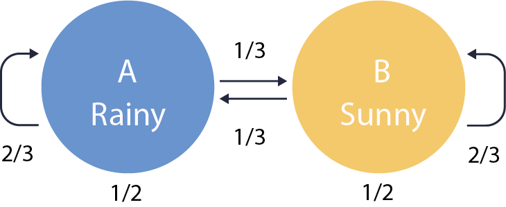
The weather stays the same with probability ⅔ and changes with probability $\frac{1}{3}$ . The probability transition matrix P is then defined as

$$\textbf{P}=\begin{bmatrix} \frac{2}{3} & \frac{1}{3}\\ \frac{1}{3} & \frac{2}{3} \end{bmatrix}$$

To fulfill the axioms of probability entries across each row should add up to one. The numbers shown below each state of the Markov Chain above are the stationary distribution. Therefore, according to our model, if today the weather is sunny in San Diego than on average the day after tomorrow will also be sunny.

More complicated, precise, and useful Markov models arise when we define the transition probabilities between nodes to be dependent on other factors. The Hidden Markov Model is just such a defined model.